Speculative Decoding: Unlocking Faster Inference in Transformers
Welcome to The Neural Nook! In this inaugural blog post, we will be exploring Speculative Decoding, an algorithm for faster decoding in transformers.
Large Language models (LLMs) generate text one token at a time (Transformer Decoding). While these models can be effectively trained on huge amounts of data, they are not very efficient at the time of inference. It's like having a super fast car, but being stuck in traffic – the model gets slowed down because it has to wait for each token to be generated before it moves to the next one. As these models get bigger, it's like the road getting narrower, causing more delays. And, if the model is spread across many devices, it's like adding more cars to the traffic jam, making things even slower.
Transformer decoding relies heavily on memory bandwidth, where the size of model parameters and memory affect the time to predict a token. As model parameters increase, so does the challenge. In this blog post, I'll walk you through Speculative Decoding, an algorithm that accelerates transformer decoding by enabling the generation of multiple tokens from each transformer call, thus significantly reducing the latency arising due to the sequential generation.
Speculative Decoding
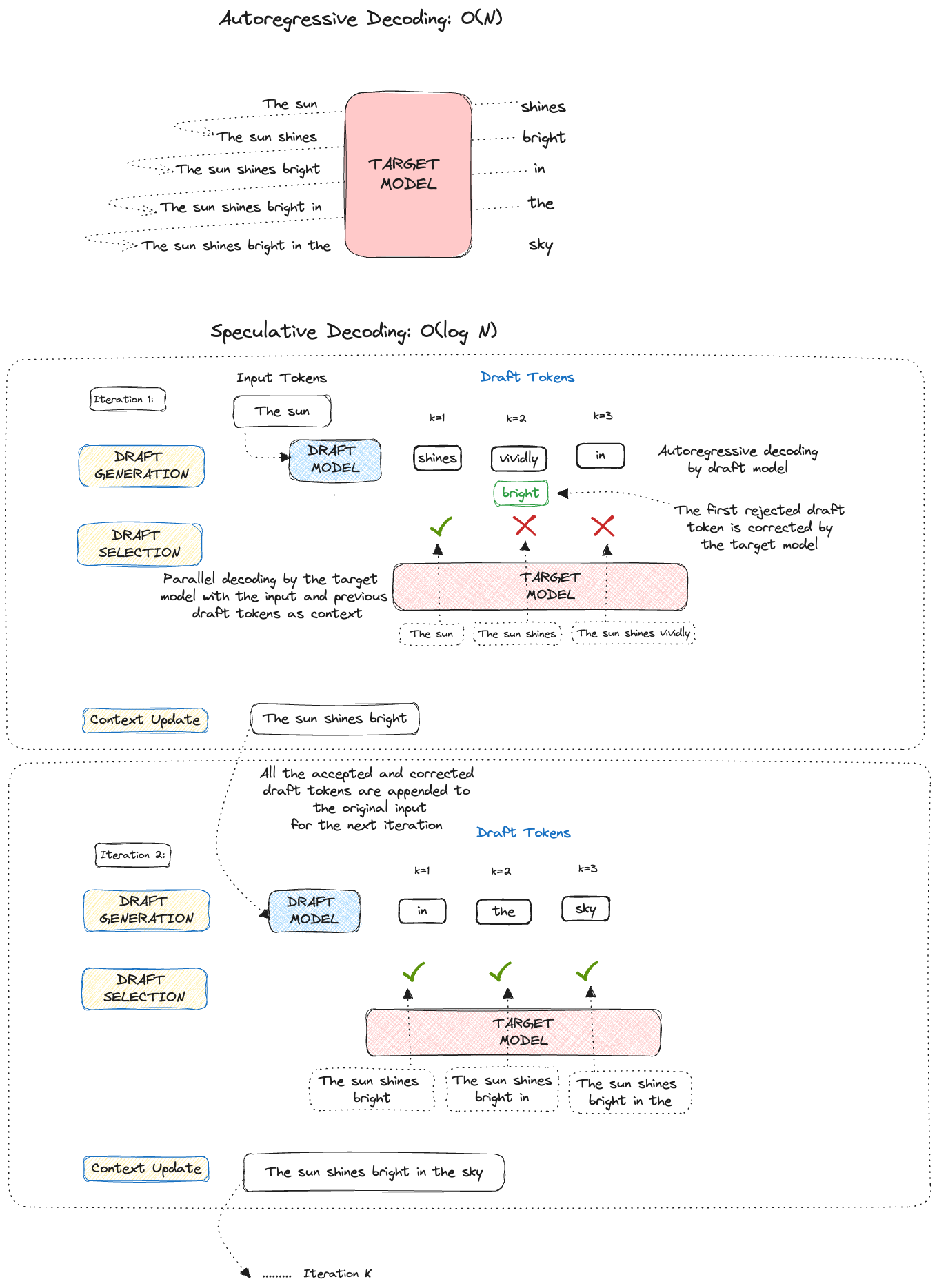
We’ll begin by providing a high-level overview of the speculative decoding algorithm's operation. Each iteration comprises the three primary steps mentioned below:
1. Draft Generation: As a first step, a smaller (faster) LLM is called K times, to generate K draft tokens. These are like educated guesses made by a smaller draft model. Choosing the right draft model gives us good-quality draft tokens.
2. Draft Selection: The generated draft tokens are scored in parallel using the larger, more powerful target model, the model from which we wish to sample. The score is used to decide whether a draft token is accepted or rejected.
3. Context Update: After accepting a subset of the 𝐾 draft tokens, the updated context is fed to the draft model for the next iteration, repeating step 1.
The success of this algorithm is based on the observation that the latency of parallel scoring of short drafts is comparable to that of sampling a single token from the larger target model.
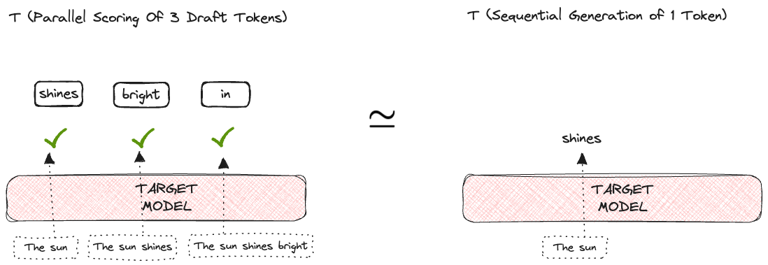
Don’t worry if all of this sounds confusing. This was just a high-level overview of what we will cover in detail in the subsequent sections of the post. Let's delve deep into each of the steps mentioned above.
Draft Generation
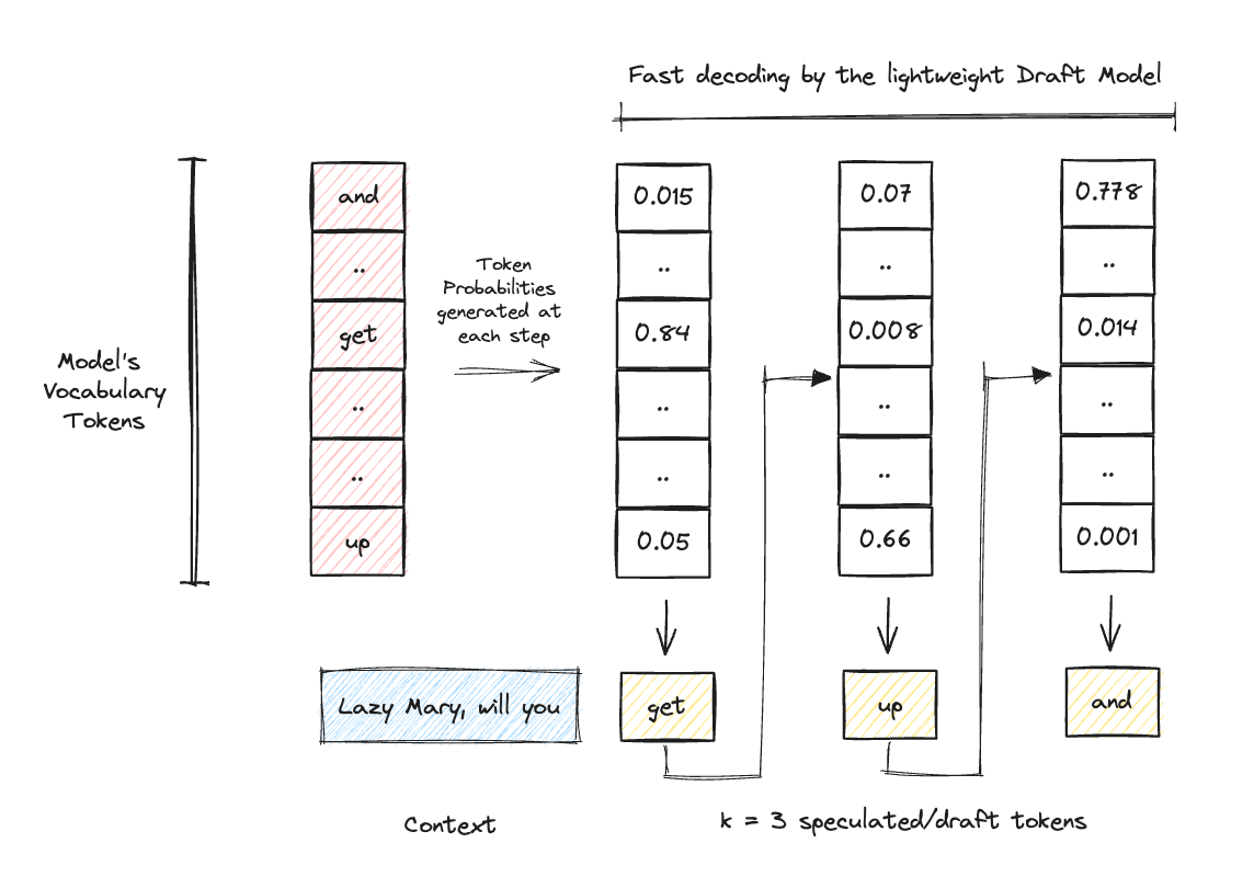
As our first step, we chose a small draft model that quickly generates the K draft tokens.
Choosing the draft model
Speed v/s Accuracy Tradeoff: Our main focus is to make the draft generation as quick and accurate as possible. A bad-quality draft model would mean that all the effort of the target model goes into correcting the generated draft tokens, which would result in no benefit overall and an extra cost for the draft model. But if we focus a lot on improving the quality of the generated draft tokens, it might lead to very slow draft generation, again defeating the entire purpose of the draft model in the first place.
We gotta find the right balance here. I mean, isn't it always about finding the right balance?
Given that around three-fourths of all anticipated tokens are generally considered "easier", for example, tokens like are, is, the can be predicted accurately even with smaller models, and hence, favoring a faster model over a more precise one makes more sense here. The larger target model can subsequently verify the remaining "challenging" tokens. Using a smaller version of the target model could be sufficient for generating drafts with high acceptance rates.
Tokenization: Firstly, the draft model should have the same tokenizer (vocabulary) as our target model. This is because as we’ll see further, the draft selection step requires comparing the draft model generated logits to that generated by the target model for each time step in the sequence. If these do not have the same tokenizer, this comparison would require additional expensive calculations.
Once we are done with choosing the draft model, the next step is to run a forward pass on the model and generate a specific number of draft tokens (K = 3 in the example below).
Draft Selection
Now, we have our draft tokens, but before incorporating them into the final output, it is crucial to ensure that they are accurate. For that, we turn to our target model.
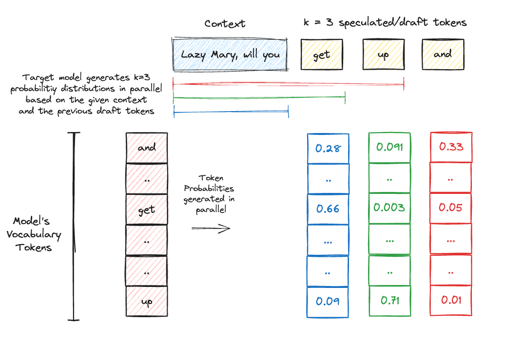
The draft tokens, along with the input sequence, are fed into the target model for scoring. This involves running K parallel forward passes through the target model. During these passes, the model considers the prior context (draft tokens for the previous positions) of each position in the sequence.
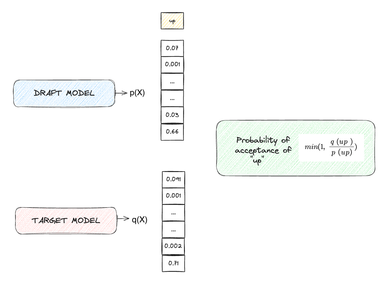
Once the target model generates the probability across the model’s vocabulary for all these K positions, the probability of the draft token as generated by the draft model is compared to the probability for the same token as per the target model’s generated probability distribution. Yes read it once more and don’t worry, we have the algorithm covered in detail below.
Rejection Sampling
For each of the draft tokens, a random variable r is sampled from the Uniform Distribution U[0,1]. The value of r decides if the draft token is accepted/rejected. Consider the following:
The draft token is accepted, only when r<Z. This leads us to the following two cases (consider the draft token up ):
Case 1: The target model is more or equally confident about the draft token as the draft model
In this case, q(up)≥p(up), implies Z=1 which means P(r<Z)=1 because r falls between 0 and 1. Therefore, the draft token is always accepted.
Case 2: The target model is less confident about the draft token than the draft model
In this case, q(up)<p(up), and we calculate Z=p(up)/q(up), where the value of Z decides if the token will be accepted or rejected. When the target model predicts the draft token with high confidence (leading to Z→1), the probability of r<Z increases, resulting in a higher probability of acceptance of the draft token. Conversely, if Z→0 (indicating p(up)≫q(up)), the token is more likely to be rejected, which makes sense intuitively.
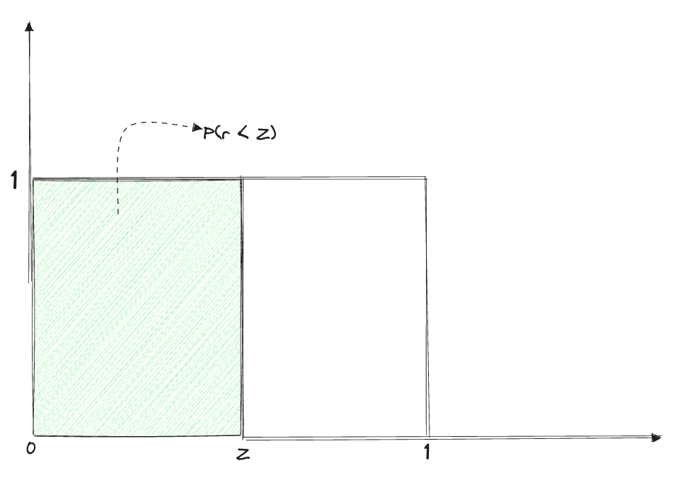
Using the rejection sampling schema mentioned above, we either accept or reject each of the K draft tokens. Once we reject a draft token, say at the ith position, all the draft tokens following it are automatically invalidated as they were generated assuming the rejected token to be correct.
Context Update
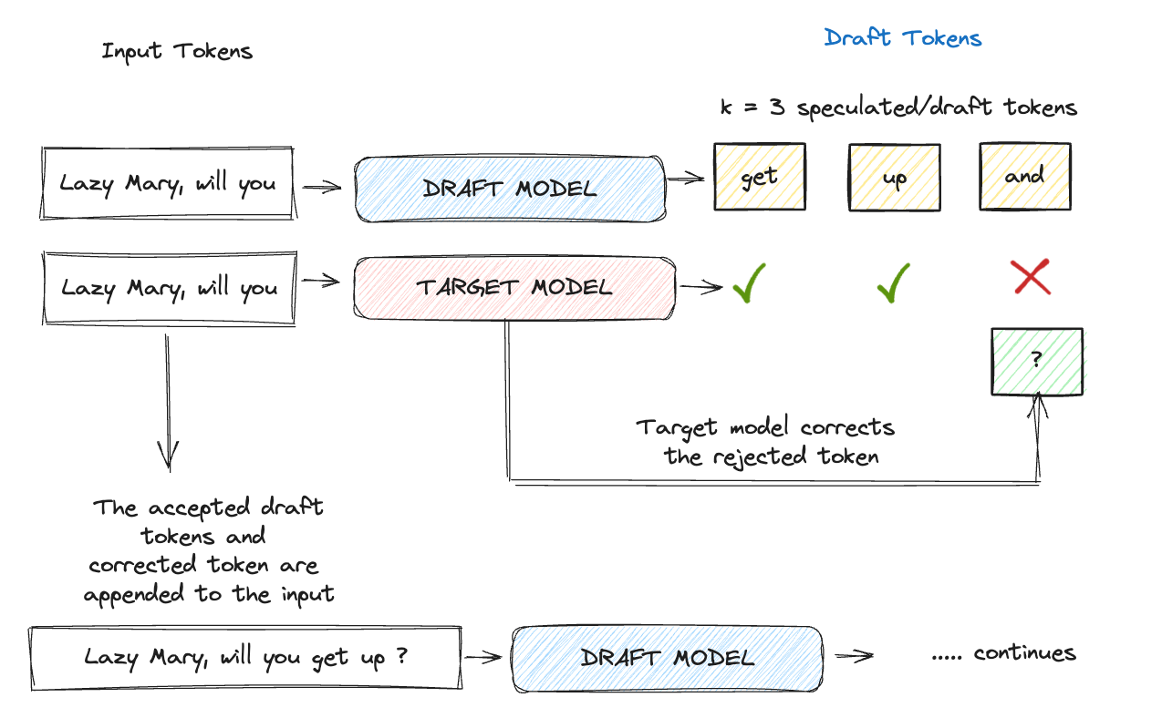
In this final step,
If all the draft tokens are accepted, the accepted draft tokens appended to the input make the new context for the next iteration.
If a draft token, say at position i, is rejected (implies all the tokens following it are also rejected), the accepted draft tokens + the target model’s prediction for the ith position is appended to the original input.
This updated context is used for querying the draft model again to predict the next K draft tokens and this process repeats iteratively. It can be seen that even if the draft model gets its token rejected at a few positions, the parallel scoring calls by the target model significantly reduce the latency (Olog(n)) and at the same time ensure the accuracy of the generated tokens.
Tuning K
We can optimize this entire process by tuning the number of draft tokens (K) generated by the model. This can be done by tracking the acceptance rate of these draft tokens, i.e. increase K if all the tokens get accepted and decrease it otherwise.
Conclusion
In this blog post, we have discussed the problems leading to the high inference times in LLMs and how speculative decoding, an innovative strategy, accelerates transformer decoding without compromising the quality of the generations. By identifying the culprit as the memory bandwidth-bound nature of the decoding and finding a way to utilize the available memory for faster generation (without tweaking any model parameters or the architecture), this strategy has demonstrated high speedups while ensuring the same outputs by using the original target model alone.
References



Clear and crisp article written Shreya.
Can you check if this is correct?
"In this case, q(up)<p(up), and we calculate Z=p(up)/q(up)"
I think Z should be equal to q(up)/p(up)